The present tutorial we will go step-by-step to
build from scratch without the use of the Geometry Editor, run and
analyze the results of a simple FLUKA simulation.
Basic knowledge of FLUKA is required.
Time needed for this tutorial: XXX h
We will simulate the neutron production and energy deposition of a
proton beam hitting a lead target similar to the old
n_TOF spallation target at
CERN.
The target had a rectangular shape of 80x80x60 cm3 and it was
submerged in a water container with a ~5 cm layer of water that was used
both for cooling and moderation. The neutrons were produced by a
20 GeV proton beam, impacting with 10º angle on the horizontal
plane.
The user must make a choice on the coordinate system. The
general tendency is to use the Z-axis collinear with the beam
axis (usually lying on the horizontal plane), and then select
the vertical and horizontal axis. In this example we will use
the following convention:
X – horizontal axis, pointing to the left, with respect to beam direction
Y – vertical axis, pointing upwards
Z – beam axis, usually horizontal
Using the
Geometry Editor
for building the geometry is the strongly recommended way of working
but this is covered in another tutorial.
Flair is an evolving project therefore some options, menus,
forms or dialog might not be exactly the same or might be replaced
by similar functionality
Solution:
tutorial.flair
In this chapter we will be starting a new flair project using the FLUKA

basic
template
-
Launch flair by typing the following command
$ flair
or from the system application menu 
Flair
$ flair -h offers a short help page for all
available command line arguments of flair. Some can be very
useful like:
- -1 open the first flair project in the current directory.
- -r open the last opened flair project
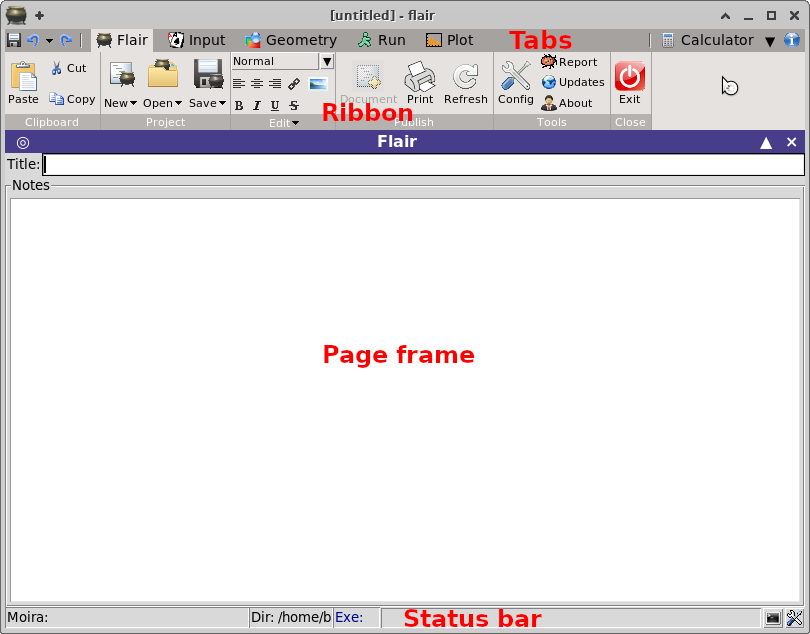
On the flair main window one can find:
-
Select the Flair tab (if it is not selected).
-
Click on the button with the new icon
 to create a new input file based on the basic template.
User templates are located in the user directory ~/.flair/templates
-
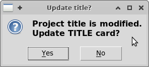
In the title entry field, type a title like:

An information dialog box will appear asking if you want to
update the TITLE and
GEOBEGIN cards inside the
FLUKA input using the title that
was entered in the project. Click yes and automatically all
FLUKA cards that require a title
string will be set with the project title.
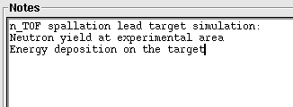
-
add also a small note describing the present project
-
Finally click on the save
 icon on the left of the tab bar.
Save it as tutorial.flair preferably save it under a new directory.
Please use this name to be consistent in all the following commands.
icon on the left of the tab bar.
Save it as tutorial.flair preferably save it under a new directory.
Please use this name to be consistent in all the following commands.
You can create directories directly in the save dialog there is a dedicated
button for it.
Control-S key is a shortcut for save
Now we will edit the input building the nTOF target geometry.
-
Select the

Input
The page below will show the input editor.
The editor will contain the default basic template, with the TITLE card filled with our Project title. The selected cards
are highlighted with a Light Yellow background color, while the active card has
a thick black border around it.
We start editing the file by going through one by one the input cards:
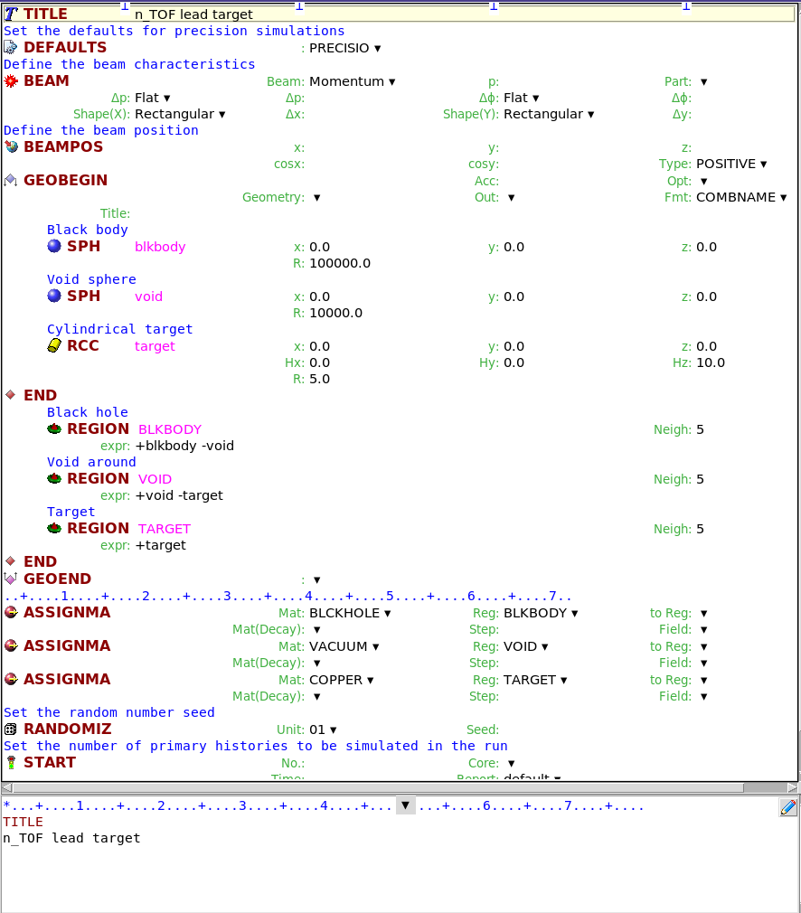
Card anatomy and terminalogy:
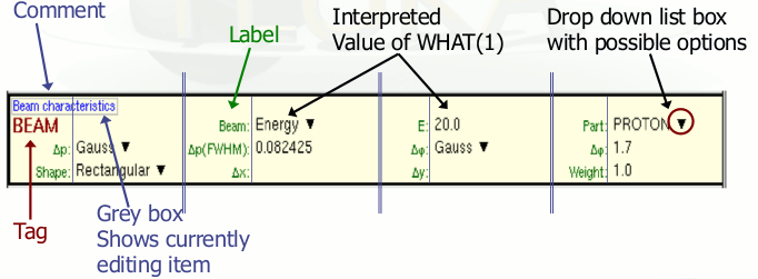
To select a card click with the mouse the Tag.
If you click on any label or value it will select the card and
start editing the value directly
You can select
multiple cards. They will be highlighted with yellow
and the active will have a black border.
warning
When you have multiple selected cards any change in the active will be
copied to ALL selected cards
During input editing there are two modes:
- Card mode where you can manipulate the
cards as a single object: i.e. Drag and drop, move,
delete, insert, copy, paste...
- Field editing mode, to modify the contents of a card.
..
To start editing the fields of a card, first select the card with
the mouse or the arrows. Click Enter to start
the field editing mode. To exit editing press
Escape-key, and you will return to Card mode.
Everything in flair is fully customizable,
colors, fonts etc.
Go to the

Preferences
,
easily accessible at the bottom-right button of the status bar.
-
Select the BEAM card by clicking on the name of the card.
Edit the card to look like the following:
 Start editing either by pressing Enter-key or by clicking with the mouse on the appropriate field. Use the
Tab-key to move to the next field:
Start editing either by pressing Enter-key or by clicking with the mouse on the appropriate field. Use the
Tab-key to move to the next field:
- Label Beam select Energy as beam type.
The next label will change to E:
- Label E: type 20 at the beam energy, meaning 20 GeV
- Label Part: select PROTON as particle type
- Label Δp select Gauss as momentum distribution
- Label Δp(FWHM) enter 0.082425 as momentum spread (GeV/c)
- Label Δφ select Gauss as angular distribution
- Label Δφ(FWHM) type 1.7 as the angular spread in mrad
You will notice that the card display at the bottom of the screen will start
to fill in with the values you typed, highlighting with yellow
the changes from the previous state. Flair always converted the numbers into
floating point format using the best representation of the number to ensure
the maximum accuracy.
All flair list boxes are searchable. Type-in the starting characters of the item you
are searching and the closest match will be selected
Hovering the mouse over the various fields displays a short help, the
default values and the units of each field.
At any time you can hit F1 to consult the manual for the active card
-
Fill up the BEAMPOS card with the following values:

We are defining a beam hitting at the location [2.2632, -0.5, -10]cm
with a direction of 10° on the horizontal plane.
To use expressions in the fields you need to start with the = character.
Look the flair manual for the valid expressions and the limitations.
Expressions can be useful for creating more readable input using units,
trigonometric expressions etc.
- Select the Geometry node on the input tree (Left frame)
to de-clatter the display.
The input editor will show only the cards belonging to the geometry
group.
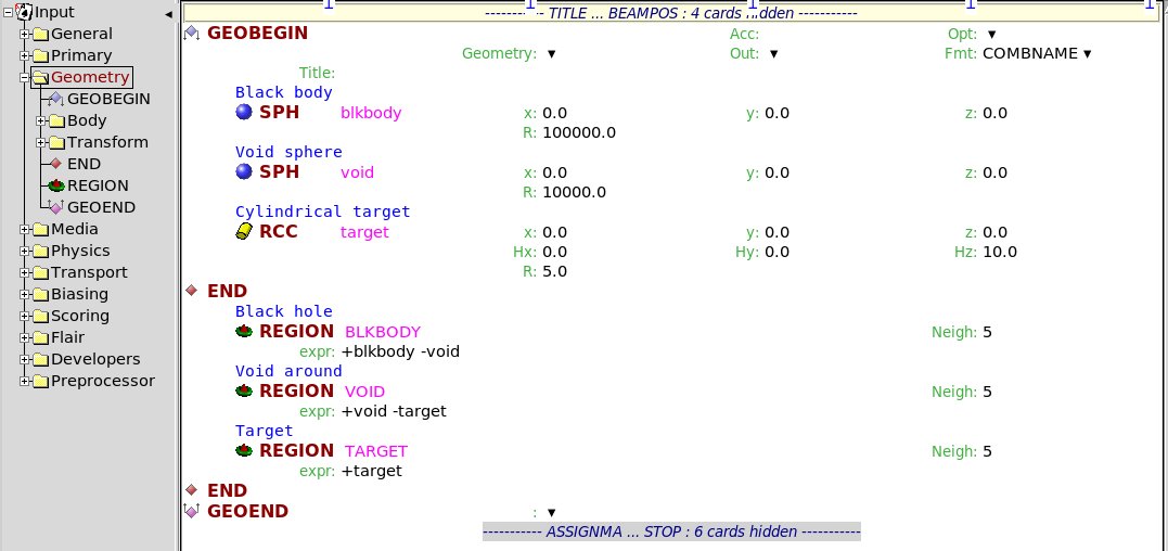
The basic template generated a default geometry consisting of two
concentric huge spheres named blkbody and
void, and a cylindrical target named
target.
In the next steps we will replace the target by a right parallelepiped named
watercnt and add two parallelepipeds named
pbtarget and niche
-
Select the card RCC target
either by clicking on it or using the Up/Down keys
-
Select from the Ribbon the command

Change ▼
Geometry → Body →  RPP
RPP
The above command will convert the RCC to RPP
WARNING: The Change commands will change the type
of card, while at the same time it tries to keep as much as possible from the
whats/fields. All exceeding whats in the new type will be discarded.
-
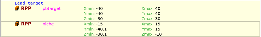
Edit the body to:
- Change the comment to Water container
- Change the body name to watercnt

When changing a body name, region, material, or detector all cards
referring to this name will be changed as well.
-
Create two new RPP bodies.
Either by right-clicking and selecting
 Geometry → Body →
RPP
Geometry → Body →
RPP
or from the Ribbon or by hitting Control-Enter or Ins
Another way would be to duplicate the current RPP hitting
Control-d or with the 
Clone
To add a comment on a card, right click the card and select
Insert Comment or from
the
Ribbon select the
 Comment ▼
.
Or with the shortcut
Control-M even simply
c
Is always a good practice to avoid touching (co-planar) bodies in
FLUKA. Either try to cut the bodies with the use of infinite
planes, or slightly overlap the bodies and then performing the appropriate logical
operation in the region definition.
-
Select the REGION TARGET
and change the comment and expression as below

Hitting the
+,
-,
Insert; keys or the icon
while editing a
REGION's expression shows a list of bodies
to select from. Press the
Escape key if you are not interested in adding any
body. This behavior can change from the configuration panel.
Lists in flair are search-able. Type the beginning of the item you are looking for and
the closest match will be highlighted. Ctrl-N or Ctrl-G repeats the last
search
-
Add a new REGION named WATERCNT
and edit it as below

To re-order the cards you can
Drag and Drop them with the mouse, or using
the
Control-Up/Down keys or from the
Ribbon with the

Move Up

Move Down
-
Select the Media item on the Input tree on the left side to edit
the material assignments to the two REGIONs
TARGET and WATERCNT
as follows:

Materials can be created either manually with the cards
MATERIAL and
COMPOUND
or import them from the
Material database accessible on the
Ribbon as

Material ▼
- Select the Scoring from the Input tree
-
Add some scoring cards
one USRBIN, and
two USRTRACKs as shown
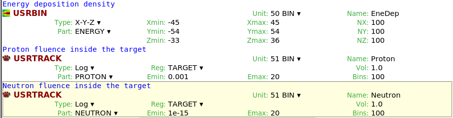
We are selecting as output file BINary since they are the only files we can later process
to merge the statistics. The ASCii files cannot be further processed with the standard
tools of FLUKA.
-
Set some primary particles in the START card for a test
run. The START card can be found in the Input Tree under the
Primary group

-
Press Control-S key to save the project
We will briefly visualize the geometry and try to navigate in the 3D space using the
geometry editor
-
Click on the

Geometry
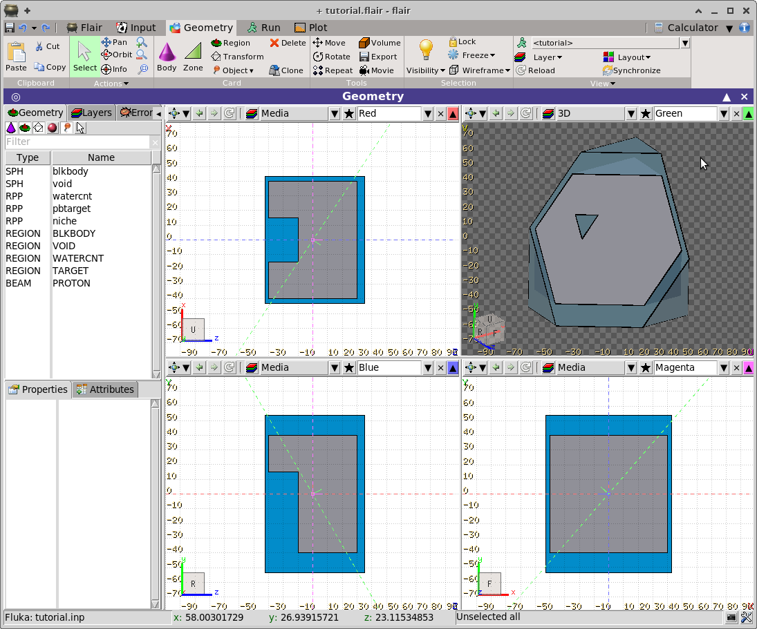
The geometry editor is extremely powerful tool for building, debugging and visualizing
the geometry and data. Please follow the dedicated tutorial to understand how it works.
At this moment all we want to see is that the geometry looks correct and there is no error or
warning displayed that needs to be addressed.
Using the
Middle mouse button and a combination of
Shift,
Control keys you can navigate very quickly in the geometry.
- Panning press and hold the Middle mouse button in any
viewport and drag the mouse.
- Set pivot point click once the Middle mouse button the
viewport will center to this location and set it as a pivot point for
the rotations
- Orbit press Control and the Middle mouse button
the viewport will rotate. Useful only when displaying in 3D. It should
be used with Setting the pivot point
- Zoom In/Out rotate the Wheel of your mouse
- Pan Backward/Forward press Control and rotate the mouse
Wheel
- Orientation Cube hover the Mouse over the orientation cube
on the bottom-left corner of each viewport. The cube will become bigger
and interactive. Click at any location, or the colored axis to change
the orientation of the viewport and or align the axis
-
As an exercise go to the green viewport
which shows the geometry in 3D.
Hover the mouse over the Orientation cube on the bottom-left corner.
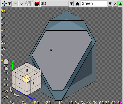
-
Click on the highlighted corner of the cube as in the above image.
The plot will be oriented facing from 45° azimuthal and 45° polar angle.
-
Press & hold the Control and rotate the mouse Wheel towards you, until you see the complete
geometry. This action moves the viewport position backwards from the screen.
-
In case you get lost you can can go back to the previous viewport locations using the
 and
and  arrows on the private toolbar
of the viewport.
arrows on the private toolbar
of the viewport.
-
In case you want to reset the viewport click the Home button in the Orientation cube
and/or the Origin button depicted as a circle.
-
Press Control-S key to save the project
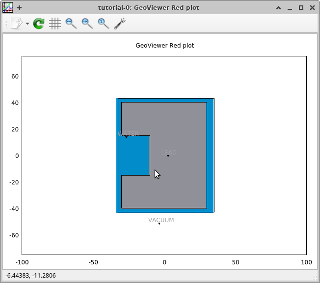
In this chapter we will use the FLUKA plotting capabilities to visualize the geometry as FLUKA will
understand it. Flair is using a different geometry kernel from FLUKA, so it is good sometimes to verify that
fluka understands correctly as in flair the geometry.
-
Select the

Plot
If you have selected the geometry tab before
the plot window will be populated with 4 geometry plots corresponding to the 4 viewports of the
Geometry editor.
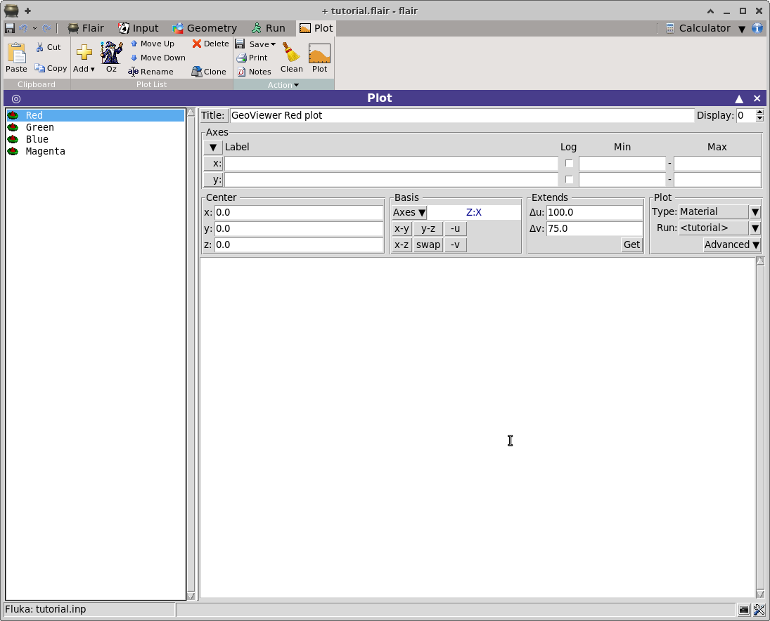
-
Click on the
 red
red
-
Click the

Plot
it will prepare a temporary input file with only the necessary information
to plot the geometry, execute FLUKA with this temporary input file and display the plot
with the use of Gnuplot as plotting engine.
Control-Enter shortcut executes the default action on each tab. Run for running, Plot for
plotting etc.
Flair as a "makefile" checks the validity of each file based on the creation time with respect
to its dependencies. For example the plot depends on the fluka output which depends on the
temporary input file which depends on the input, If something has changed in between it will
try to re-calculated only what it is needed. If for some reason it fails, it is a good habit to
press the
 Clean
Clean button and force recalculation of everything.
-
Press Control-S key to save the project
We are ready now to launch a FLUKA run and monitor its progress
-
Select the

Run
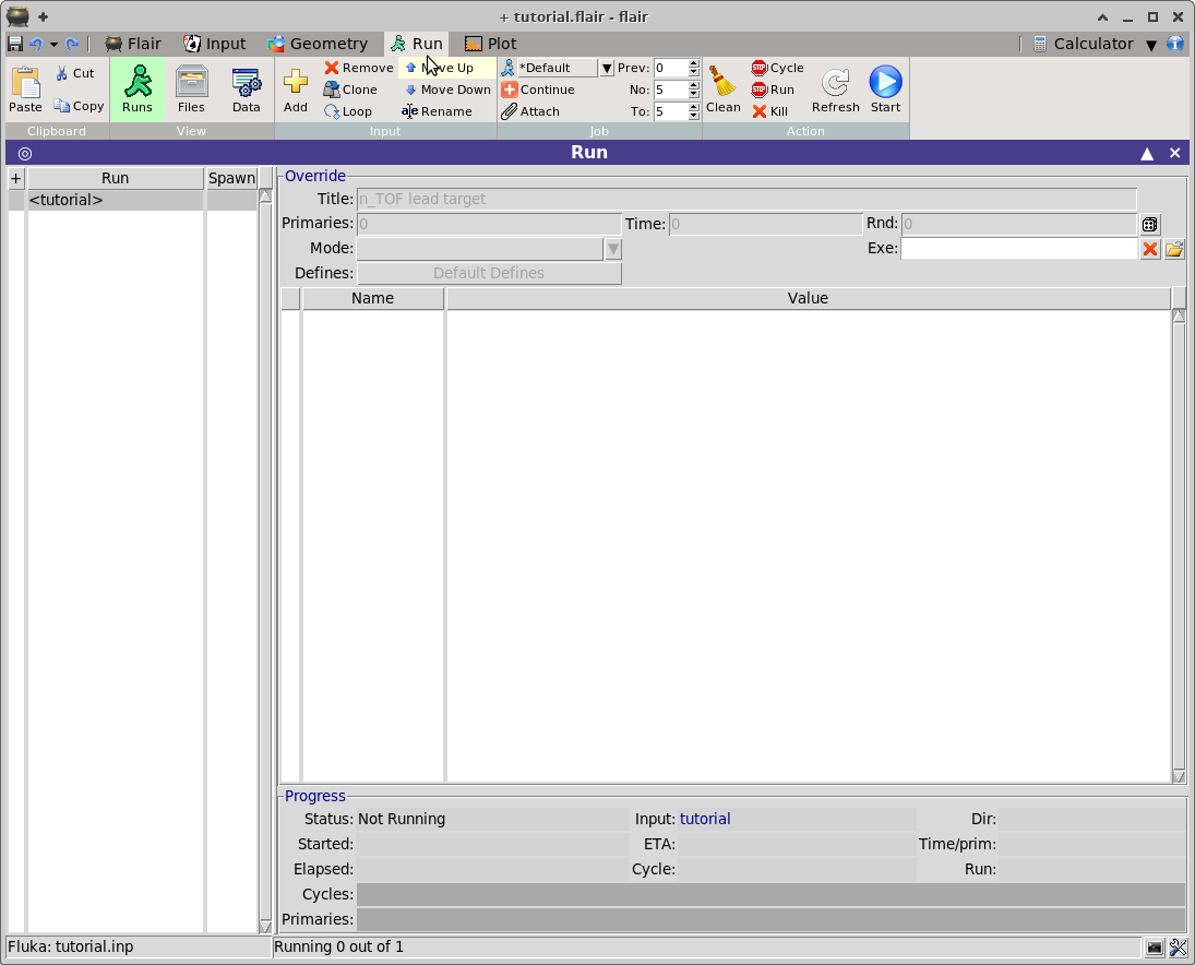
The listbox on the left shows all the runs that are associated with the current input file.
The first entry <tutorial> inside the angle-brackets <> corresponds to a run
using the input *AS IS*.
The user can create clones of the run modifying some parameters like the title,
primaries, random number seed, operation mode and as well #define variables
For the moment we are going to run the input as is
To run on a multicore machine enter the number of CPUs you want to use in the Spawn
column of the run list. It will create one separate run for each CPU.
-
Select the <tutorial> if it is not selected and click
 Start
Start
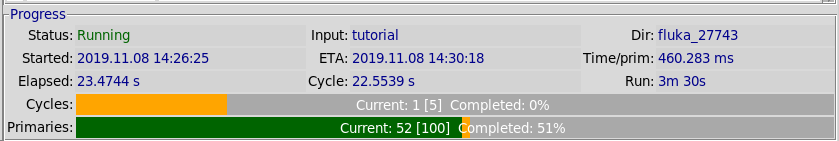
You should see the progress of the run at the dialog below like in the image.
Flair by default will submit 5 cycles as defined with the
Prev: No: and To: fields on the Ribbon.
The refreshing takes place every few seconds but if for some reason it stops you can always
press the
 Refresh
 button.
During the execution the “Status” will change, initially to Waiting to attach, followed
by Running and finally in Finished OK.
The run is submitted using the defined submit program (the default is nohup). The program
is running decoupled from the flair editor, therefore if you click save on the project and exit
the program. The next time you will open the program, flair will try to attach and display the
current run status.
Flair is trying to peek the run information by looking the status of the output files. It
doesn't make use of the system process information. This way it increases portability across
different platforms, and batch systems (see the qfluka.sh example for a substitution of
the submit command). Flair will be able to monitor the status only if the run takes place on the
same directory. The drawback of this method is that takes some time to attach.

Cycle
Run

Kill

Attach
-
Press Control-S key to save the project
-
Wait until the simulation finishes. It will take a few minutes.
During the
FLUKA run or when a cycle is completed, the user can inspect and/or
delete the output files generated by
FLUKA from the
Run:Files sub-page
-
Selecting the
Run
 Files
Files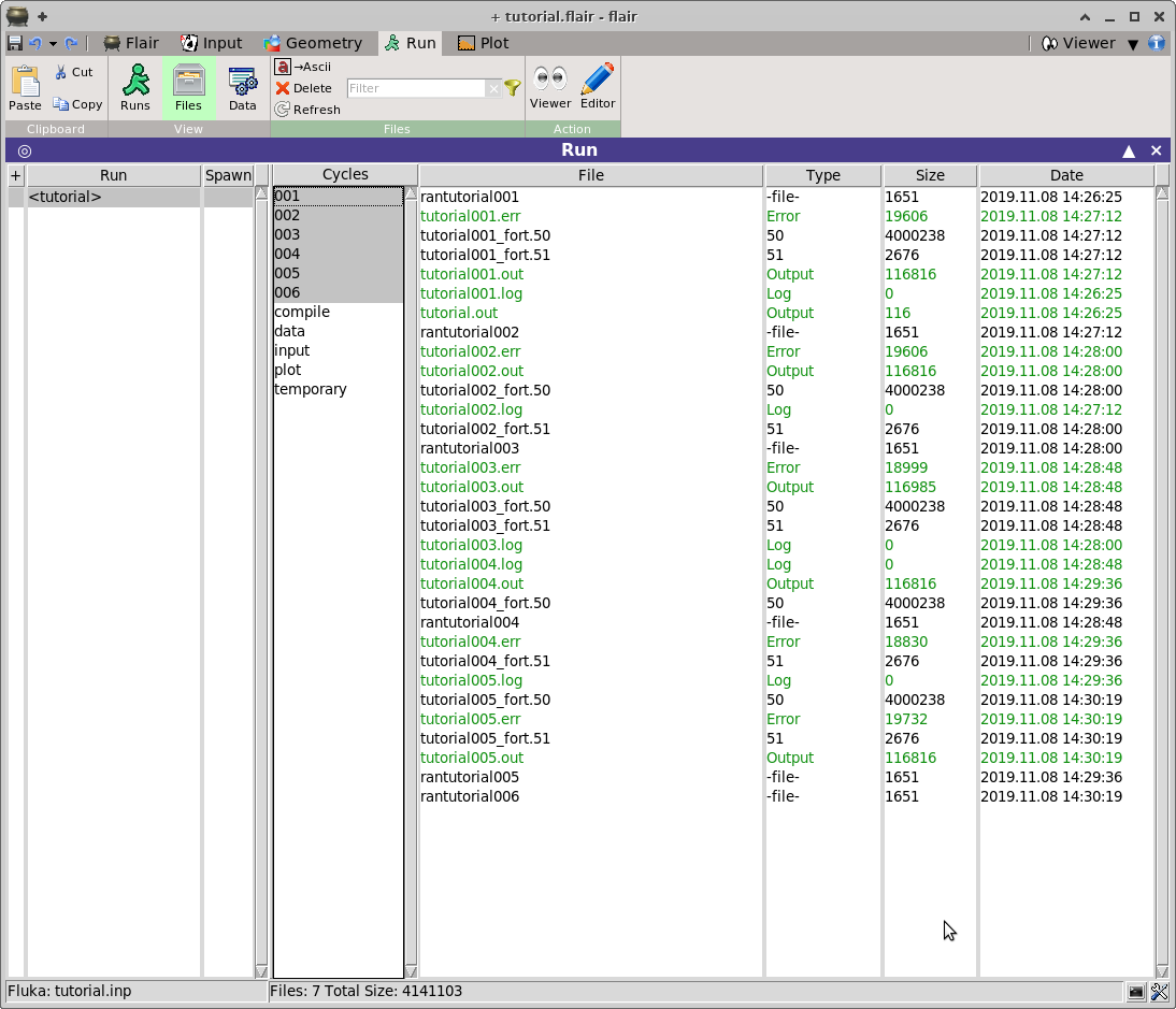 The page is composed by 3 list-boxes.
- Run on the left the common listbox with all defined runs
- Cycles in the middle containing all the cycles
that are performed and output files exists for the specific run.
There are a few virtual cycles like compile, data, input, plot, temporary
containing files generated by other process.
- Files selecting one or many cycles the last listbox will show all the relevant
files belonging to that cycle where you can view, edit, delete, rename etc...
WARNING: Do not try to open binary files. Could be rather huge
for the editor or viewer and in any case incomprehensible.
-
Click on the file tutorial001.out and click the
 Viewer
You don't need to wait to finish the run to see the output files. You can
inspect them at any time as they are generated.
The next step is to merge the output data files of the run from the various cycles in order to create
the files contain the average values and the statistical error to be used for plotting.
A bit of theory on the use of cycles
One would expect that the simulation is equivalent to a counting experiment, therefore the data will
follow a Poisson distribution and the error will be the square root of the number of events collected.
This is true provided that no biasing is used in the simulation. When importance scoring is involved
(quite typical and recommended way of working) to calculate correctly the statistical error, apart from
the final value one has to record also the square number of events/hits (second momentum) for every
value needed. This doubles the memory and increases the complexity for special estimators. Therefore, FLUKA is making use of the Central Limit Theorem for calculating the mean value of
a quantity scored and the error on the determination of the mean. The theorem states:
The distribution of an average tends to be Normal, even when the distribution from which
the average is computed is decidedly non-Normal.
This is the main reason we have to perform several cycles, minimum 5 is recommended to simulate
correctly a Normal distribution, and then sum-up and average the results. In FLUKA this is done automatically with the us?suw utilities (where ?
can be: b=USRBIN, r=RESNUCLEi, t=USRTRACK or USRCOLL, x=USRBDX,
y=USRYIELD). These programs expect as input a list of binary files generated from FLUKA with the respective card and using as unit a negative number, and in the end
they generate a set of output files both binary, text and tabulated with the results.
Flair makes this process transparent to the user with the Process Data page.
-
Select the Run:Data tab page
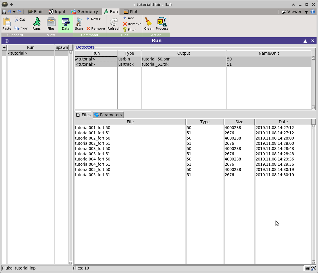
-
Normally flair should detect all scoring cards and create the appropriate data
merging rules.
To re-scan all detectors: select all
Detectors from the top listbox and click
 Scan
Scan or

Remove
which will delete everything and force the re-scanning of
the input.
-
Select the detectors to process and click
 Process
The
FLUKA utilities usually generate more than one output files.
Typically the merge binary data file has the requested name while for a text file is
generated with the extension
_sum.lis, and a tabulated one with the extension
_tab.lis
The last step is to plot the data, we will create 2 plots one for the
USRBIN
file that contains the energy deposition on the spallation target, one for the
USRTRACK estimators with the particle fluences.
-
Select the
Plot
-
Click on the wizard button
 Oz
Oz

tutorial_50_plot

tutorial_51_plot
Normally the plots are ready to be plotted but lets fine tune them
-
Select in the list the
tutorial_50_plot
-
Fill in the values as you see in the following image.
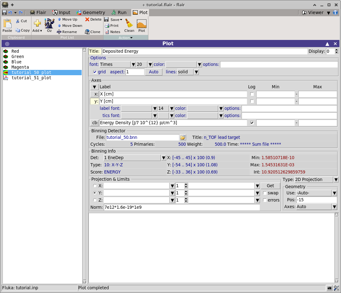
- Title: enter the plot title
- Title: clicking the title shows additional configuration options like font,
color...
- Detector click on the button and select the tutorial_usrbin_50 file we
created in the Data page. Automatically the run and detector information in the file
will be filled.
- Projection & Limits select projection on the Y-axis without supplying
any limits. This will generate a projection from -54 to +54cm on the XZ plane.
- Norm select as normalization the formula “7e12*1.6e-19*1e9”, this way
every value will be converted from GeV/cm3/p to
J/cm3/pulse where a pulse has 7e12 protons.
Advanced options are hidden and can be enabled by clicking the relevant LabelButton
like the
Title: or
x:...
Once clicked additional options will appear
You can edit multiple plots at the same time. When you will select more than one plots the
common fields will be displayed and will be by default DISABLED (Grayed out).
With the mouse Right click on the field and it will enable it. All fields that are
enabled will propagate their value as is to all selected plots.
-
Clicking on the
Plot
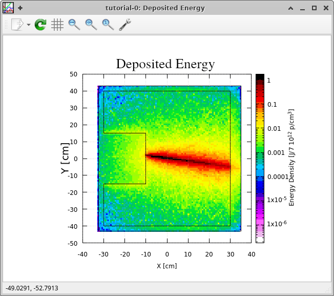
- Once the plot is created you can save it as image by clicking the
Save ▼ drop down list and select the file type.
Note that the
Save ▼ is located in
the
Ribbon close to the
Plot button.
The save buttons on the ribbon acts only for the current displayed tab page
and not for the flair project.
Prefer to use the .eps format for higher quality figures.
The scoring cards
USRBDX,
USRCOLL,
USRTRACK,
USRYIELD
after the data merging are producing a single differential quantities that can be plotted with the
“USR-1D” plot frame in flair. This frame is using the
_tab.lis file and many data can be super
imposed one on top of the other.
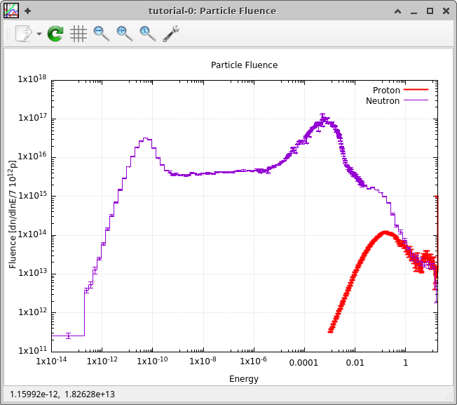
- Select the
tutorial_51_plot
- Fill in the values as you see in the following image.
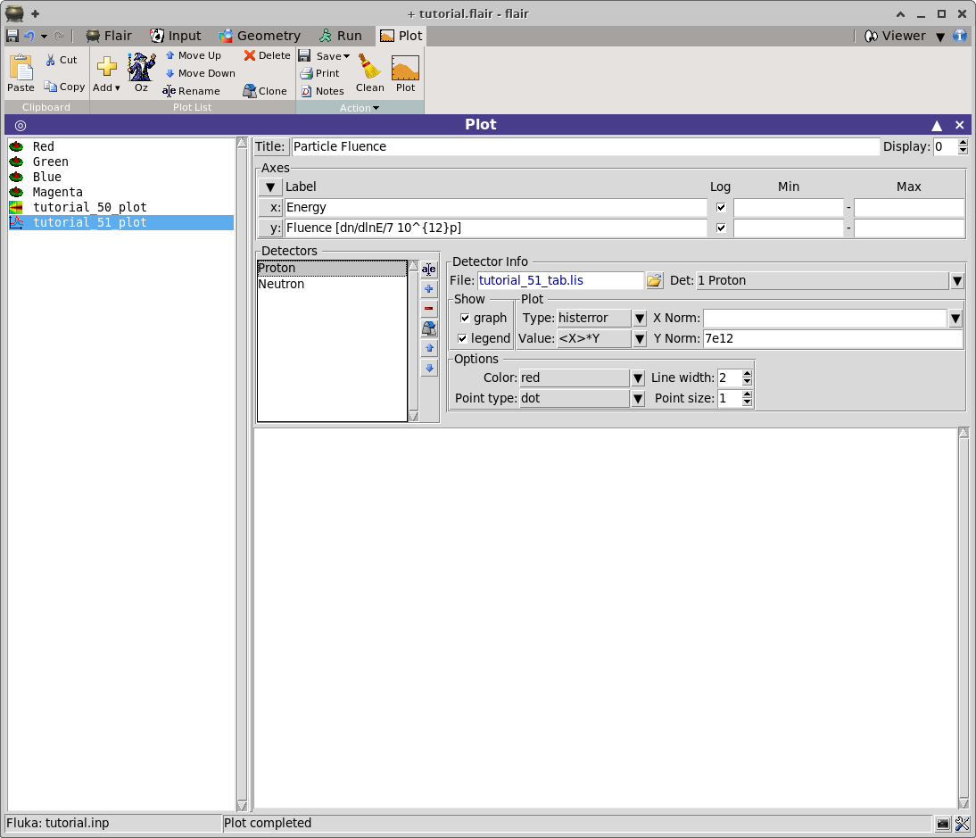
- Be careful to tick the Log for the X and Y axes
- Rename the Detector 1 to Proton and select the Det: 1 Proton ▼
- Clone the Proton detector with Ctrl-D or with the button
- Rename the cloned detector to Neutron and select Det: 2 Neutron
- Select both detectors Proton and Neutron. All the fields will be disabled (grayed
out).
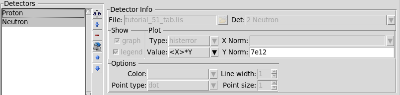
- Right click on the Value: and select the <X>*Y. You are selecting
Iso-lethargic way of plotting
- Right click on the Y Norm: and type in 7e12 as the normalization for both detectors
- Click on the Proton and on the Neutron to verify that the plotting value and the
normalization are properly taken for both
- Click on the
Plot
-
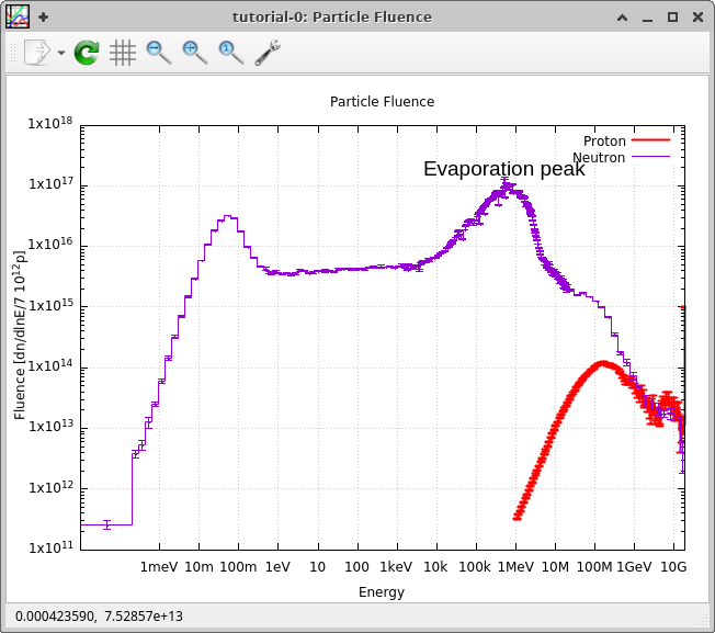
Optionally you can customize even more the plot using the commands big text box below,
issuing directly gnuplot commands
							set xtics ('1meV' 1e-12, '10m' 1e-11, '100m'
									1e-10, '1eV' 1e-9, '10' 1e-8,'100' 1e-7,'1keV' 1e-6, '10k' 1e-5,
									'100k' 1e-4, '1MeV' 1e-3, '10M' 0.01, '100M' 0.1, '1GeV' 1, '10G' 10,
									'100G' 100, '1TeV' 1000, '10T' 1e4, '100T' 1e5)

							set label 'Evaporation peak' at 5e-6,2e17 font 'Arial,14'
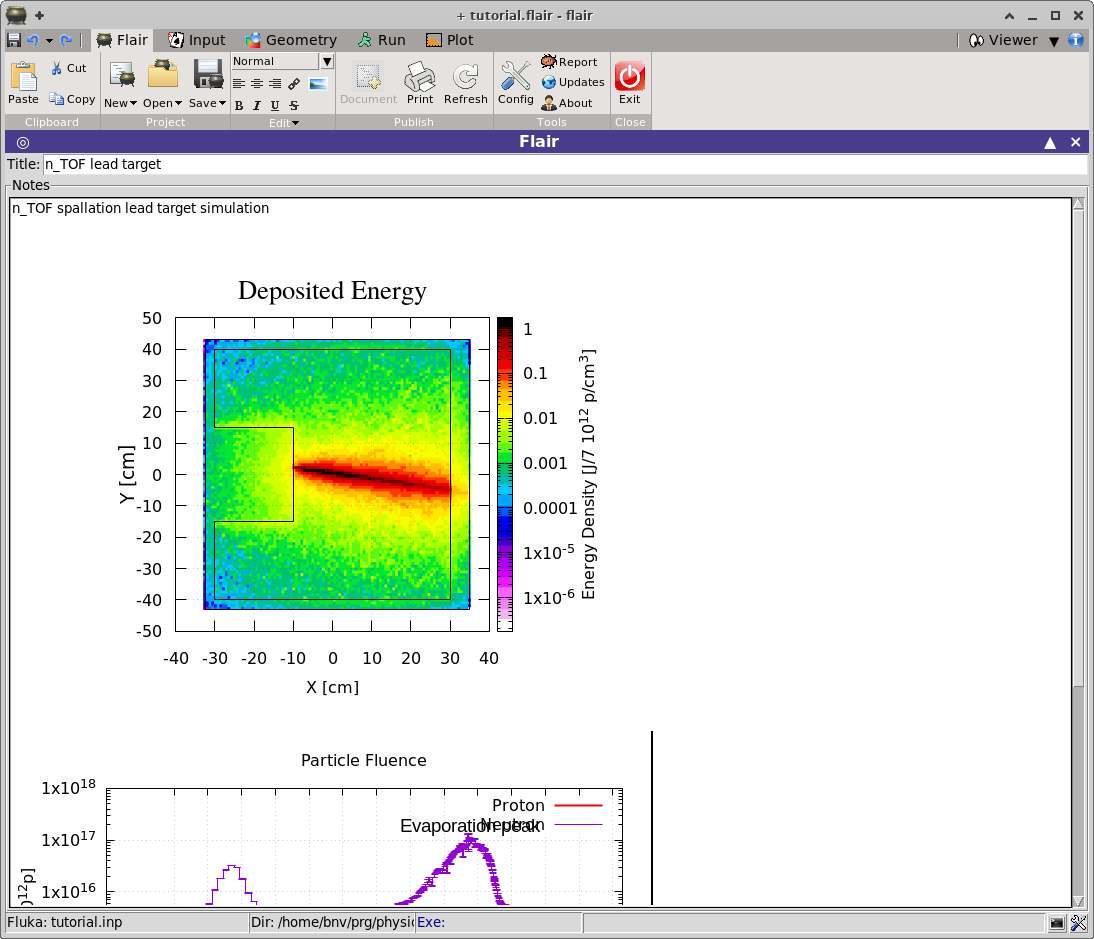
- Finally you can "push" the plots to the Project notes page of the
Flair
tutorial_50_plot
tutorial_51_plot
and click the 
Notes
-
Select the
Flair
The project note page should look like
-
Press Control-S key to save the project
 flair
flair